R code to illuatrate VIF in OLS

Remeber that the variance inflation factor (VIF) is given by

\[\hat{var}(\beta_j)=\frac{s^2}{(n-1)\hat{var}(X_j)}\times\frac{1}{1-R^2_j}\]

where \(R^2_j\) is the \(R^2\) from the regression of \(X_j\) on the other covariates.

However, when first learning about VIF is can be hard to comprehend. To make it easier some illustrations are often nice.

Below is some code to illustrate the variance inflation factor in R.

library(ggplot2)
library(reshape)
require(tikzDevice)
set.seed(32)         # Set the seed for reproducible results
sims    <- 1000          # Set the number of simulations at the top of the script
V.1      <- array(0, dim = c(sims, 3))
B.1      <- array(0, dim = c(sims, 3))
V.2      <- array(0, dim = c(sims, 3))
B.2      <- array(0, dim = c(sims, 3))
V.3      <- array(0, dim = c(sims, 3))
B.3      <- array(0, dim = c(sims, 3))
a       <- 1            # True value for the intercept
b1      <- 4            # True value for the slope
b2      <- 2
n       <- 100           # sample size

p <- 0.1
for(i in 1:sims){               # Start the loop
  u<-rnorm(n, 0, 1)
  v<-rnorm(n, 0, 1)
  x1 <- 2*u*+2
  x2 <- 2*(p*u+sqrt(1-p^2)*v)+2
  Y <- a + b1*x1+b2*x2 + rnorm(n, 0, 1) # The true DGP, with N(0, 1) error
  model <- lm(Y ~ x1+x2)            # Estimate OLS Model

  B.1[i,] <- model$coef             # store coefficients
  V.1[i,]<-sqrt(diag(vcov(model)))  # store variance
}

p <- 0.5
for(i in 1:sims){               # Start the loop
  u<-rnorm(n, 0, 1)
  v<-rnorm(n, 0, 1)
  x1 <- 2*u*+2
  x2 <- 2*(p*u+sqrt(1-p^2)*v)+2
  Y <- a + b1*x1+b2*x2 + rnorm(n, 0, 1) # The true DGP, with N(0, 1) error
  model <- lm(Y ~ x1+x2)            # Estimate OLS Model
  B.2[i,] <- model$coef             # store coefficients
  V.2[i,]<-sqrt(diag(vcov(model)))  # store variance
}                               # End loop

p <- 0.9
for(i in 1:sims){               # Start the loop
  u<-rnorm(n, 0, 1)
  v<-rnorm(n, 0, 1)
  x1 <- 2*u*+2
  x2 <- 2*(p*u+sqrt(1-p^2)*v)+2
  Y <- a + b1*x1+b2*x2 + rnorm(n, 0, 1) # The true DGP, with N(0, 1) error
  model <- lm(Y ~ x1+x2)            # Estimate OLS Model
  B.3[i,] <- model$coef             # store coefficients
  V.3[i,]<-sqrt(diag(vcov(model)))  # store variance
}                               # End loop

B1 <- data.frame(B.1)
V1 <- data.frame(V.1)
B1$corr <- "A"
V1$corr <- "A"

B2 <- data.frame(B.2)
V2 <- data.frame(V.2)
B2$corr <- "B"
V2$corr <- "B"

B3<- data.frame(B.3)
V3 <- data.frame(V.3)
B3$corr <- "C"
V3$corr <- "C"

B <- rbind(B1,B2,B3)
V <- rbind(V1,V2,V3)


tikz('densityb1.tex',standAlone=FALSE, width=4,height=2.5)
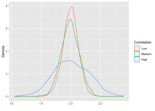
ggplot(B, aes(x=X2, colour=corr)) +
  geom_density()+
  scale_colour_discrete(name  ="Correlation",
                        breaks=c("A", "B","C"),
                        labels=c("Low", "Medium","High"))+
  xlab("") +
  ylab("Density")
dev.off()


ggplot(B, aes(x=X3, colour=corr)) +
  geom_density()+
  scale_colour_discrete(name  ="Correlation",
                        breaks=c("A", "B","C"),
                        labels=c("Low", "Medium","High"))+
  xlab("") +
  ylab("Density")